這篇文章講資料的基本處理。主要用到的就是
tidyverse套件系統。它提供了資料科學的一些實用的函式。
我們首先要安裝 tidyverse 套件系統。
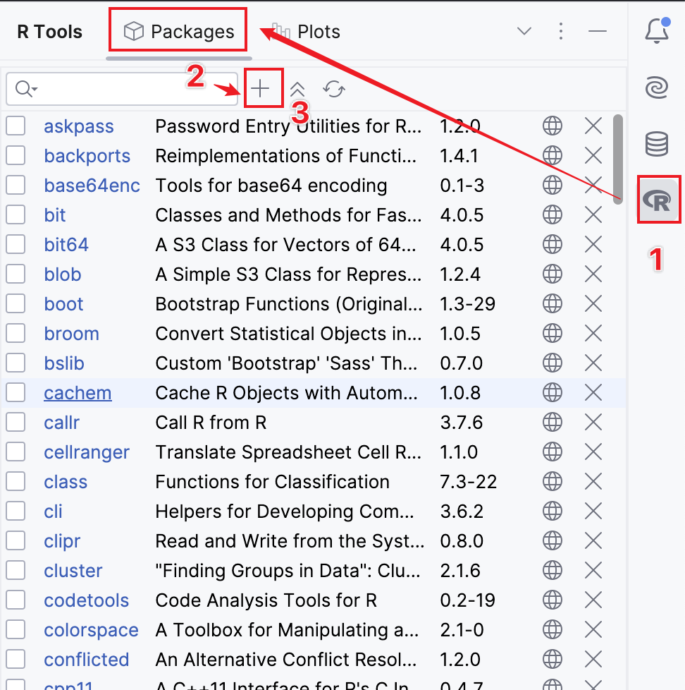
install.packages("tidyverse")如果是第一次安裝套件,會讓你選擇 CRAN repository 的 mirror,就近選擇一個就好。我是有選擇台大的鏡像站。另外,如果你想要更換鏡像站的話,在 PyCharm 下的步驟如下:
- 打開側邊欄 R Tools,切換到 Packages。
- 點按上面的“+”。
- 點按 Manage Repositories。
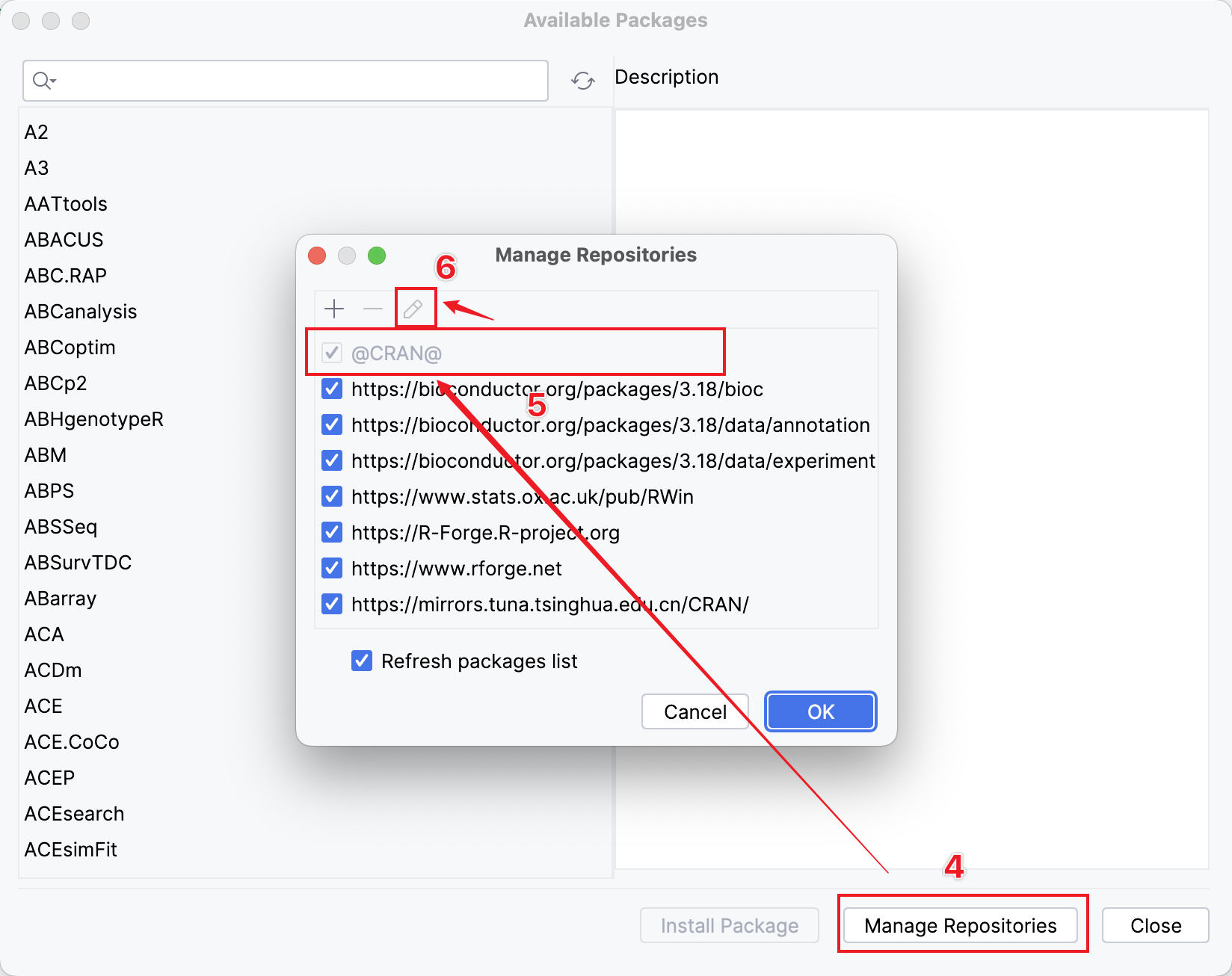
- 在彈出的視窗中點按 @CRAN@,然後點按上面的筆形按鈕。
- 在彈出的視窗中選擇 Repository。

在 R Studio 中的步驟請自行 Google。
資料輸入
資料輸入套件 readr
readr 是 tidyverse 套件系統中的一個套件,專門用於處理資料的輸入。其中的函式有 read_csv() 用於輸入 .csv 資料檔, read_excel() 輸入 excel 資料檔,read_delim() 輸入不同分隔符號的資料檔。
其中 read_delim() 函式的定義如下:
read_delim( file, delim, quote = "\"", escape_backslash = FALSE, escape_double = TRUE, col_names = TRUE, col_types = NULL, locale = default_locale(), na = c("", "NA"), quoted_na = TRUE, comment = "", trim_ws = FALSE, skip = 0, n_max = Inf, guess_max = min(1000, n_max), progress = show_progress(), skip_empty_rows = TRUE)解釋一下引數:
- file:路徑與檔名
- delim:分隔符號
- quote:視同分隔符號(資料的文字變數值常放在雙引號中)
- escape_backslash:預設 FALSE,是否有逃脫符號
- escape_double:預設 TRUE,是否用引號符號作為逃脫符號
- col_names:設定變數名(T 或 F)
- col_types:設定變數的類型
- na:設定 NA 符號
- comment:設定注釋符號,在注釋符號之後的文字不會被讀入
- trim_ws:去除變數值得空白
- skip:要跳過幾行(row)才開始讀入資料
- n_max:最大輸入行數
library(tidyverse)library(readr)dd <- readr::read_csv("./Data/DMTKAInfMo.csv")
library(readxl)dd <- readxl::read_excel("C:/RData/DMTKAInfMo.xls")整潔資料
所謂整潔資料(tidy data),可以認為是一個使用 R 進行處理的資料標準。該標準的基本要求如下:
- 每個變數各自形成一欄(縱行, column)
- 每個列(橫列, row)各自為一個觀測時間的測量
- 一個檔案只用一張資料表(sheet)
- 一個欄位(縱行, Column)只有一個變數,同時有清楚的變數名
- 若完整資料包含不同資料表,則不同資料表要有索引(inxex)或指標變數(id)可進行關聯與串聯
Tibble與Data Frame
透過 readr 套件讀入的資料會被儲存成 tibble 物件。它相較於 data.frame 幾乎無差別,只是多了一些方便 tidyverse 處理的屬性。
使用 as.data.frame() 函式可以將 tibble 物件轉成 data.frame。使用 as_tibble() 函式也可以將 data.frame 轉換成 tibble。
資料流動管道運算指令
運算指令為 %>%,稱為 pipe,由 tidyverse 套件系統中的 magrittr 套件提供。
運算指令的左側通常是資料物件,包括資料框架、矩陣、向量等。右側則通常是函式。在流動過程中,左側的資料物件自動成為右側函式的第一個引數。
library(magrittr)c(1:10) %>% mean() %>% log()## [1] 1.705## 相當於 log(mean(c(1:10)))資料檢視函式 glimpse()
在讀入資料之後,我們必須對資料進行檢視,從而確定資料是否有被正確讀入。在 tidyverse 套件系統的 tibble 套件中提供一個檢視資料的函式 glimpse(),該函式類似於 R base 中的 str()。
執行效果如下:
glimpse(dd)## Rows: 137## Columns: 8## $ treat <fct> placebo, placebo, placebo, placebo, placebo, placebo, placebo, pla...## $ cellcode <fct> squamous, squamous, squamous, squamous, squamous, squamous, squamo...## $ time <int> 72, 411, 228, 126, 118, 10, 82, 110, 314, 100, 42, 8, 144, 25, 11,...## $ censor <fct> dead, dead, dead, dead, dead, dead, dead, dead, dead, survival, de...## $ diagtime <int> 60, 70, 60, 60, 70, 20, 40, 80, 50, 70, 60, 40, 30, 80, 70, 60, 60...## $ kps <int> 7, 5, 3, 9, 11, 5, 10, 29, 18, 6, 4, 58, 4, 9, 11, 3, 9, 2, 4, 4, ...## $ age <int> 69, 64, 38, 63, 65, 49, 69, 68, 43, 70, 81, 63, 63, 52, 48, 61, 42...## $ prior <fct> no, yes, no, yes, yes, no, yes, no, no, no, no, yes, no, yes, yes,...資料處理
資料處理的套件主要是 tidyverse 套件系統中的 dplyr 套件。用於將讀入的資料進行處理和統計操作。
選擇個體函式 filter()
從這個函式的名字也可以知道,這個函式和 JS、Java 等程式語言中的 filter 類似,都是起到一個過濾器的作用。在 Excel 中,也有類似的方法實現條件的過濾。
例如,我們想要選擇上面 survVATrial.csv 檔案內容中,threat 為 placebo,cellcode 為 large 的內容:
dd.a <- dd %>% filter(threat == 'placebo', cellcode == 'large')依據變數值排序函式 arrange()
預設情況下從小到大排序,如果要反排,可以使用 desc() 函式。
## 按照 age 變數從小到大排序dd.s <- dd %>% arrange(age)
## 按照 time 變數從大到小排序dd.s <- dd %>% arrange(desc(time))選擇變數或欄位子集函式 select()
透過選擇欄位,可以建立欄位子集,將需要的變數儲存起來進行分析,這樣可以大大加速分析執行速度。
## 選擇餓 dd 中 threat, cellcode, censor 三個變數dd.c <- dd %>% select(treat, cellcode, censor)變數轉換函式 mutate()
使用 mutate() 函式,可以將變數進行一定形式的變換,形成一欄新的變數。
dd.a <- dd %>% mutate( log_age = log(age), diag_age = diagtime * age / 100)三因素運算函式 if_else()
這個函式類似於C家族程式語言中的三因素運算元 ?:,其定義如下:
if_else(condition, true, false, missing = NULL)解釋:如果 condition 的值為 TRUE,回傳 true 的值,否則回傳 false 的值。missing = NULL 表示遺失值應當以什麼字元替代。
x <- -10:10if_else(x > 0, 0, 1)## [1] 1 1 1 1 1 1 1 1 1 1 1 0 0 0 0 0 0 0 0 0 0變數重新命名函式 rename()
可以將變數重新命名:
## 格式:new_name = old_namedd.new <- dd %>% rename(drug = treat)移除遺失資料 drop_na()
使用 tidyr 套件中的函式 drop_na() 可將缺失值個體移除。請注意,缺失值移除將完全移除一個個體。只要該列中任意一個變數為NA,則將該列完全移除。
## 移除所有含有缺失值的個體dd.mis %>% drop_na()
## 移除 age 變數含有缺失值的個體dd.mis %>% drop_na(age)隨機抽樣函式 sample_n()和sample_frac()
這兩個函式可以對資料進行隨機抽樣。引數如下:
- size = k:設定所要抽出之樣本數或分率。
- weight:抽取之相對應權重,若無設定,則權重相等。
- replace = FALSE:設定是否可以重複抽取。
dd %>% sample_n(size = 5, replace = FALSE)明顯不同個體選擇函式 distinct() 和 n_distinct()
舉例來說,假設你有一個資料框包含了某個學校的學生資訊,裡面有學生的姓名、性別和年級等欄位。如果有幾個學生重名,那麼使用 distinct() 函式就能快速地找出資料框中唯一不重複的學生資料列。
使用橫列指標選出個體函式 slice()
slice() 為一系列函式,可以利用橫列指標(row index)選出個體(row)。
- slice()
- slice_head():選出資料最前端的個體
- slice_last():選出資料最末端的個體
- slice_min():選出資料變數值最小的個體
- slice_max():選出資料變數值最大的個體
- slice_sample():隨機選出個體
## 選出第一列dd %>% slice(1)
## 選出 1~3 列dd %>% slice(1:3)
## 選出 101~最後dd %>% slice(101:n())
## 選出除掉 1~100 列之後的所有列dd %>% slice(-c(1:100))
## 選出開頭三列dd %>% slice_head(n = 3)
## 選出末尾三列dd %>% slice_tail(n = 3)
## 選出 time 變數最小的三列dd %>% slice_min(time, n = 3)
## 選出 time 變數最大的三列dd %>% slice_max(time, n = 3)
## 隨機選出三列set.seed(1)dd %>% slice_sample(n = 3)計算常見統計量函式 summarise()
smmarise() 函式可以計算常見的統計量,比如個數、平均值、變異數等等,並將計算結果單獨作為一個變數插入原始資料中。
dd %>% summarise( count = n(), age_mean = mean(age, na.rm = TRUE), age_sd = sd(age, na.rm = TRUE) )資料分組操作函式 group_by()
資料分析常常需要類別變數分組,個別操作資料或進行計算統計量。函式 group_by() 引數可放入類別變數,然後分組進行相同資料分析。
dd %>% group_by(treat) %>% summarise( diagtime_mean = mean(diagtime, na.rm = TRUE), diagtime_sd = sd(diagtime, na.rm = TRUE) )## # A tibble: 2 x 3## treat diagtime_mean diagtime_sd## <fct> <dbl> <dbl>## 1 placebo 59.2 18.7## 2 test 57.9 21.4多變數計算統計量函式 summarise_all()
summarise() 函式只能分別對當一變數進行計算,若要同時對許多變數進行相同操作,可使用以下函式:
- summarise_all():對每一個變數進行相同操作
- summarise_each():對每一個變數進行相同操作, 需加變數名
- summarise_at():對選出的變數進行相同操作 需加變數名
- summarise_if():對符合特定條件的變數進行相同操作
## summarise_all()con.mean <- dd %>% select(time, diagtime, kps, age) %>% summarise_all(mean, na.rm = TRUE)con.mean## # A tibble: 1 x 4## time diagtime kps age## <dbl> <dbl> <dbl> <dbl>## 1 122. 58.6 8.77 58.3#con.sd <- dd %>% select(time, diagtime, kps, age) %>% summarise_all(sd, na.rm = TRUE)con.sd## # A tibble: 1 x 4## time diagtime kps age## <dbl> <dbl> <dbl> <dbl>## 1 158. 20.0 10.6 10.5id <- c("mean", "sd")comb <- rbind(con.mean, con.sd)comb <- cbind(id, comb)comb## id time diagtime kps age## 1 mean 121.6 58.57 8.774 58.31## 2 sd 157.8 20.04 10.612 10.54#dd %>% select(time, diagtime, kps, age) %>% summarise_all(list(mean, sd), na.rm = TRUE)## # A tibble: 1 x 8## time_fn1 diagtime_fn1 kps_fn1 age_fn1 time_fn2 diagtime_fn2 kps_fn2 age_fn2## <dbl> <dbl> <dbl> <dbl> <dbl> <dbl> <dbl> <dbl>## 1 122. 58.6 8.77 58.3 158. 20.0 10.6 10.5dd %>% select(time, diagtime, kps, age) %>% summarise_all(lst(mean, sd), na.rm = TRUE)## # A tibble: 1 x 8## time_mean diagtime_mean kps_mean age_mean time_sd diagtime_sd kps_sd age_sd## <dbl> <dbl> <dbl> <dbl> <dbl> <dbl> <dbl> <dbl>## 1 122. 58.6 8.77 58.3 158. 20.0 10.6 10.5dd %>% summarise_each(list(mean, sd), time, age) # not so useful## Warning: `summarise_each_()` is deprecated as of dplyr 0.7.0.## Please use `across()` instead.## This warning is displayed once every 8 hours.## Call `lifecycle::last_warnings()` to see where this warning was generated.## # A tibble: 1 x 4## time_fn1 age_fn1 time_fn2 age_fn2## <dbl> <dbl> <dbl> <dbl>## 1 122. 58.3 158. 10.5dd %>% summarise_each(lst(mean, sd), time, age) # not so useful## # A tibble: 1 x 4## time_mean age_mean time_sd age_sd## <dbl> <dbl> <dbl> <dbl>## 1 122. 58.3 158. 10.5dd %>% summarise_at(c("time", "age"), mean, na.rm = TRUE)## # A tibble: 1 x 2## time age## <dbl> <dbl>## 1 122. 58.3dd %>% summarise_at(.vars = vars(time, age), mean, na.rm = TRUE)## # A tibble: 1 x 2## time age## <dbl> <dbl>## 1 122. 58.3dd %>% summarise_at(.vars = vars(time, age), .funs = c(Mean = "mean", SD = "sd"), na.rm = TRUE)## # A tibble: 1 x 4## time_Mean age_Mean time_SD age_SD## <dbl> <dbl> <dbl> <dbl>## 1 122. 58.3 158. 10.5dd %>% summarise_if(is.numeric, list(mean, sd), na.rm = TRUE)## # A tibble: 1 x 8## time_fn1 diagtime_fn1 kps_fn1 age_fn1 time_fn2 diagtime_fn2 kps_fn2 age_fn2## <dbl> <dbl> <dbl> <dbl> <dbl> <dbl> <dbl> <dbl>## 1 122. 58.6 8.77 58.3 158. 20.0 10.6 10.5dd %>% summarise_if(is.numeric, lst(mean, sd), na.rm = TRUE)## # A tibble: 1 x 8## time_mean diagtime_mean kps_mean age_mean time_sd diagtime_sd kps_sd age_sd## <dbl> <dbl> <dbl> <dbl> <dbl> <dbl> <dbl> <dbl>## 1 122. 58.6 8.77 58.3 158. 20.0 10.6 10.5資料聯集與交集函式
- intersect():交集
- union():并集
- setdiff():差集
tibble1 <- tibble( id = c(1, 2, 3, 4, 5), name = c("Alice", "Bob", "Charlie", "David", "Emily"))tibble2 <- tibble( id = c(3, 4, 5, 6, 7), name = c("Charlie", "David", "Emily", "Frank", "George"))
## 二者交集intersect(tibble1, tibble2)## # A tibble: 3 × 2## id name## <dbl> <chr>## 1 3 Charlie## 2 4 David## 3 5 Emily
## 二者并集union(tibble1, tibble2)## # A tibble: 7 × 2## id name## <dbl> <chr>## 1 1 Alice## 2 2 Bob## 3 3 Charlie## 4 4 David## 5 5 Emily## 6 6 Frank## 7 7 George
## 二者差集setdiff(tibble1, tibble2)## # A tibble: 2 × 2## id name## <dbl> <chr>## 1 1 Alice## 2 2 Bob資料合併函式
資料經常儲存再不同檔案,例如門診檔,住院檔,實驗室檔,同一位個體常須使用個體辨識碼(id)或姓名(names)進行合併或清理。用來連結不同資料的個體辨識碼或變數稱為“關鍵碼”或“所引鍵”(key)。
在 tidyverse 套件系統中,有一些函式可以實現這樣的合併作業。
- inner_join(x, y):包函 x 與 y 都配對存在的 y 與 y 個體與變數
- left_join(x, y):包函所有 x 個體與變數且在 y 有配對存在的 y 個體與變數
- right_join(x, y):包函所有y個體與變數且在x有配對存在的x個體與變數
- full_join(x, y):包函所有 x 與 y 的個體與變數資料
- semi_join(x, y):包函 x 在 y 有配對存在的 x 個體與變數
- anti_join(x, y):包函 x 在 y 無配對存在的 x 個體與變數
set.seed(1)df <- dd %>% select(treat, cellcode, time, censor, age) %>% mutate(id = 1:n()) %>% filter(id <= 10)x <- df %>% select(id, treat, time, age) %>% sample_n(size = 7, replace = FALSE) %>% arrange(id)y <- df %>% select(id, cellcode, censor, age) %>% sample_n(size = 7, replace = FALSE) %>% arrange(id)x## # A tibble: 7 x 4## id treat time age## <int> <fct> <int> <int>## 1 1 placebo 72 69## 2 2 placebo 411 64## 3 3 placebo 228 38## 4 4 placebo 126 63## 5 5 placebo 118 65## 6 7 placebo 82 69## 7 9 placebo 314 43y## # A tibble: 7 x 4## id cellcode censor age## <int> <fct> <fct> <int>## 1 1 squamous dead 69## 2 2 squamous dead 64## 3 3 squamous dead 38## 4 5 squamous dead 65## 5 6 squamous dead 49## 6 7 squamous dead 69## 7 10 squamous survival 70inner_join(x, y)## # A tibble: 5 x 6## id treat time age cellcode censor## <int> <fct> <int> <int> <fct> <fct>## 1 1 placebo 72 69 squamous dead## 2 2 placebo 411 64 squamous dead## 3 3 placebo 228 38 squamous dead## 4 5 placebo 118 65 squamous dead## 5 7 placebo 82 69 squamous deadleft_join(x, y)## # A tibble: 7 x 6## id treat time age cellcode censor## <int> <fct> <int> <int> <fct> <fct>## 1 1 placebo 72 69 squamous dead## 2 2 placebo 411 64 squamous dead## 3 3 placebo 228 38 squamous dead## 4 4 placebo 126 63 <NA> <NA>## 5 5 placebo 118 65 squamous dead## 6 7 placebo 82 69 squamous dead## 7 9 placebo 314 43 <NA> <NA>right_join(x, y)## # A tibble: 7 x 6## id treat time age cellcode censor## <int> <fct> <int> <int> <fct> <fct>## 1 1 placebo 72 69 squamous dead## 2 2 placebo 411 64 squamous dead## 3 3 placebo 228 38 squamous dead## 4 5 placebo 118 65 squamous dead## 5 7 placebo 82 69 squamous dead## 6 6 <NA> NA 49 squamous dead## 7 10 <NA> NA 70 squamous survivalfull_join(x, y)## # A tibble: 9 x 6## id treat time age cellcode censor## <int> <fct> <int> <int> <fct> <fct>## 1 1 placebo 72 69 squamous dead## 2 2 placebo 411 64 squamous dead## 3 3 placebo 228 38 squamous dead## 4 4 placebo 126 63 <NA> <NA>## 5 5 placebo 118 65 squamous dead## 6 7 placebo 82 69 squamous dead## 7 9 placebo 314 43 <NA> <NA>## 8 6 <NA> NA 49 squamous dead## 9 10 <NA> NA 70 squamous survivalsemi_join(x, y)## # A tibble: 5 x 4## id treat time age## <int> <fct> <int> <int>## 1 1 placebo 72 69## 2 2 placebo 411 64## 3 3 placebo 228 38## 4 5 placebo 118 65## 5 7 placebo 82 69anti_join(x, y)## # A tibble: 2 x 4## id treat time age## <int> <fct> <int> <int>## 1 4 placebo 126 63## 2 9 placebo 314 43